7.4 Poisson regressie

Poissonregressie werkt hetzelfde als binomiale, maar je gebruikt family = poisson. Zo simpel is dat.

Voorbeeld van data over aantal overreden amfibiën t.o.v. afstand tot een Nationaal Park in Portugal:

roadkill %>% 
  ggplot(aes(D.PARK, TOT.N)) +
  geom_point()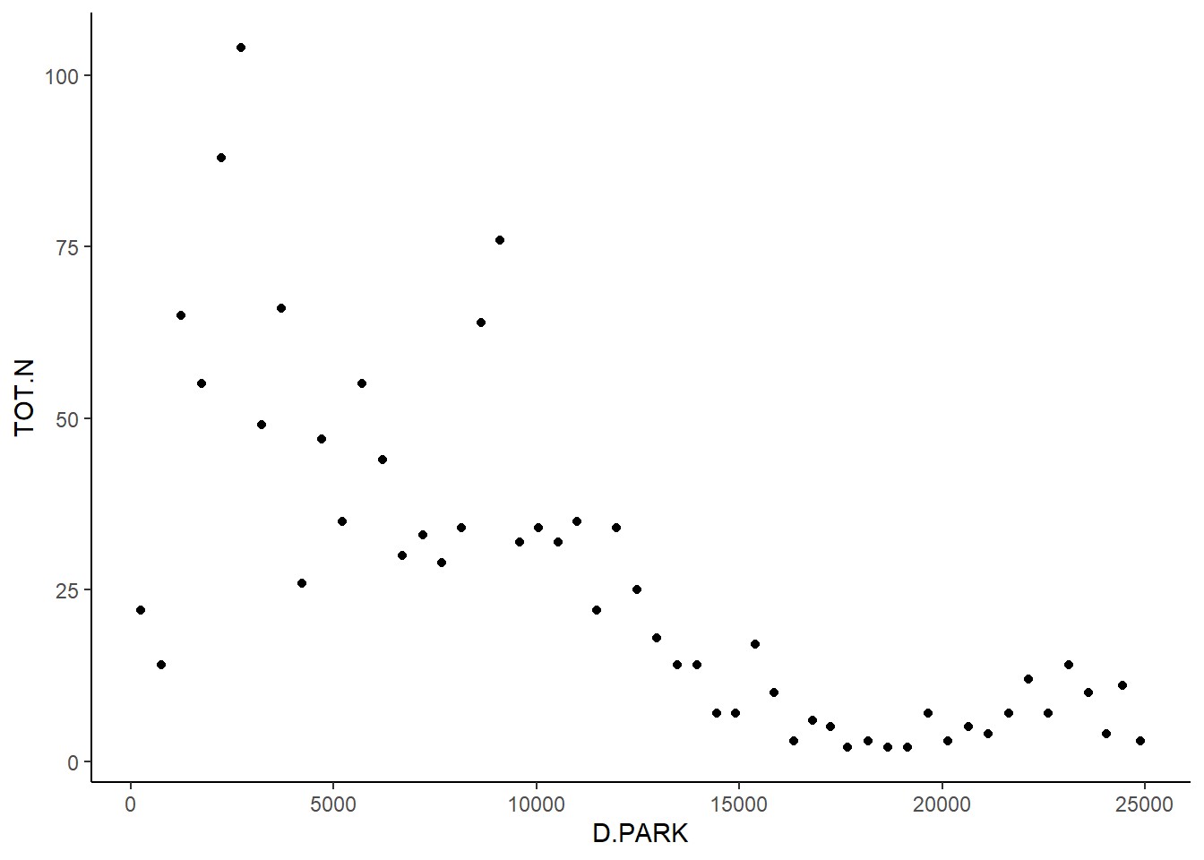

Hier kunnen we een regressie op loslaten:

fit <- glm(TOT.N ~ D.PARK, data = roadkill, family = poisson)
summary(fit)

## 
## Call:
## glm(formula = TOT.N ~ D.PARK, family = poisson, data = roadkill)
## 
## Deviance Residuals: 
##     Min       1Q   Median       3Q      Max  
## -8.1100  -1.6950  -0.4708   1.4206   7.3337  
## 
## Coefficients:
##               Estimate Std. Error z value Pr(>|z|)    
## (Intercept)  4.316e+00  4.322e-02   99.87   <2e-16 ***
## D.PARK      -1.059e-04  4.387e-06  -24.13   <2e-16 ***
## ---
## Signif. codes:  0 '***' 0.001 '**' 0.01 '*' 0.05 '.' 0.1 ' ' 1
## 
## (Dispersion parameter for poisson family taken to be 1)
## 
##     Null deviance: 1071.4  on 51  degrees of freedom
## Residual deviance:  390.9  on 50  degrees of freedom
## AIC: 634.29
## 
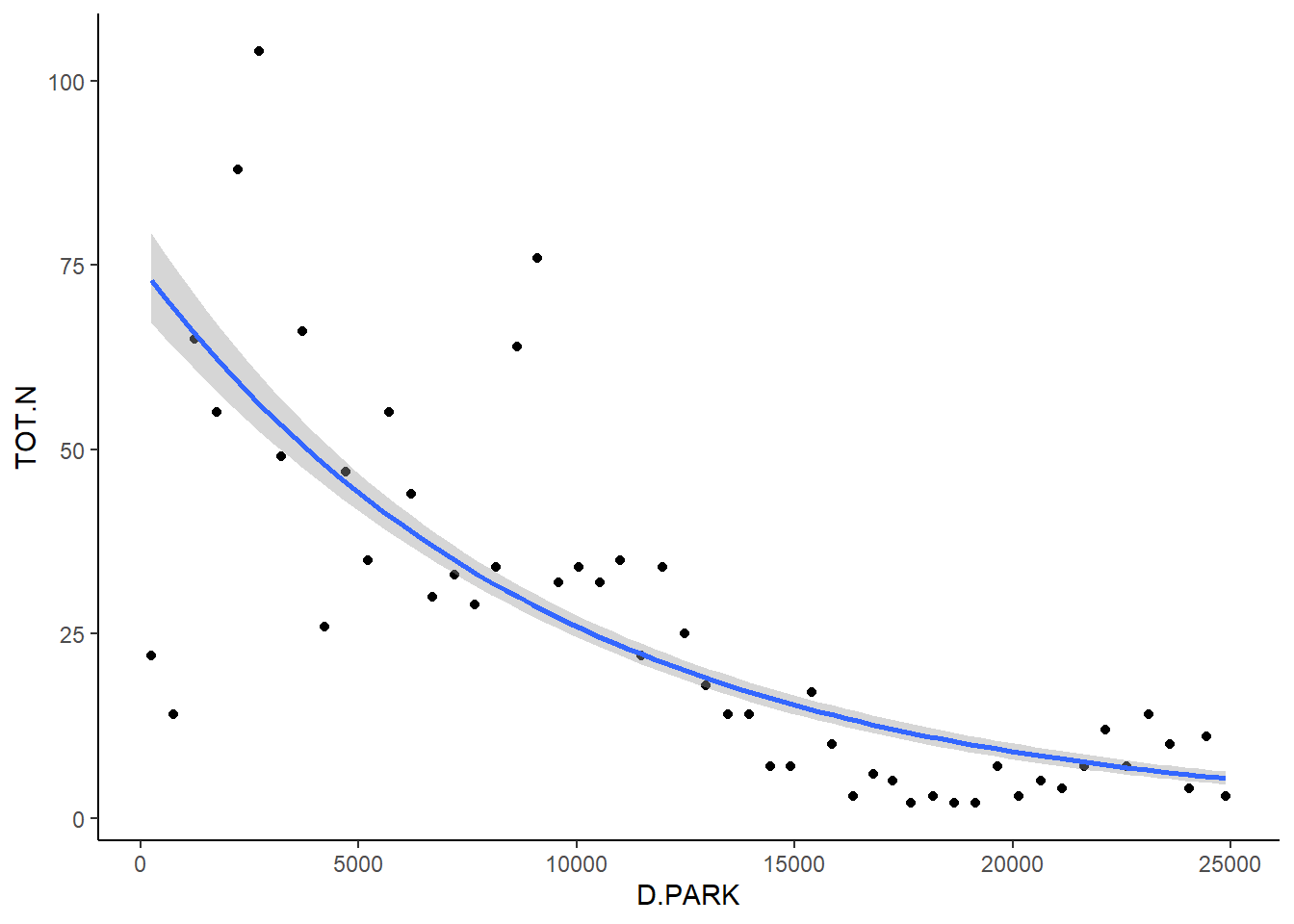
## Number of Fisher Scoring iterations: 4

Met functie geom_smooth kan je ook zulk soort modellen fitten op je data in een grafiek:

roadkill %>% 
  ggplot(aes(D.PARK, TOT.N)) +
  geom_point() +
  geom_smooth(method = 'glm', method.args = list(family = poisson))

7.4.1 Generalized Mixed Effects Models

Als je een random variabele hebt (bijv. diersoort in bovenstaand geval), dan kan je die helaas niet in de functie glm() toepassen. Dat kan wel in de functie lmer() uit de package lme4.